Table of Contents
Quantum Fourier Transform
This week's lesson will be pretty involved, as we're going to set up most of the groundwork necessary to understand Shor's algorithm, arguably the most important quantum algorithm known to date.
I want to start with a quick discussion of the continuous Fourier transform. Imagine the sound wave of some complicated chord being played. The Fourier transform allows us to decompose the notes being played by converting the "time domain" of the sound wave plotted to a "frequency domain," where each note frequency can stand out as a spike.
We will be doing something very different, but I want you to think about that example in your head as we discuss the quantum Fourier transform.
The other example I want you to think about is the Hadamard transform
$$ H^{\otimes n}|0\rangle = \frac{1}{2^{n/2}} \sum_{j=0}^{2^n-1} |j\rangle $$which is formatted very similarly to the quantum Fourier transform. While the Hadamard transform is not exactly a special case of the QFT, it is close.1
The quantum Fourier transform is a quantum operator that is defined as
$$ \text{QFT}|j\rangle = \frac{1}{2^{n/2}} \sum_{k=0}^{2^n-1} e^{2\pi ijk/2^n}|k\rangle. $$where we assume that we have a superposition of $2^n$ terms.2 It also has a useful matrix form
$$ F_n = \frac{1}{2^{n/2}} \begin{pmatrix} 1 & 1 & 1 & \cdots & 1 \\ 1 & \omega & \omega^2 & \cdots & \omega^{2^n-1} \\ 1 & \omega^2 & \omega^4 & \cdots & \omega^{2(2^n-1)} \\ \vdots & \vdots & \vdots & \ddots & \vdots \\ 1 & \omega^{2^n-1} & \omega^{2(2^n-1)} & \cdots & \omega^{(2^n-1)(2^n-1)} \end{pmatrix} $$where $\omega = e^{2\pi i/2^n}$.
This operator may seem a little cryptic for now if you're not already familiar with the Fourier transform, and that's okay. The Fourier transform as a whole has a long, pretty convergent history that I don't want to get into here.
For now, I want you to trust me that this operator will be useful to implement, and let's try to figure out a way to implement it using quantum gates.
The key gate that we will need is the controlled version of the phase gate
$$ P(\theta) = \begin{pmatrix} 1 & 0 \\ 0 & e^{i\theta} \end{pmatrix} $$which you may recognize as a generalization of the $S$ gate, which is equivalent to $P(\pi/2)$, or of the $Z$ gate, which is $P(\pi)$.
It turns out, with a bit of tensor algebra, you can rewrite the QFT formula as
$$ \text{QFT}|j\rangle = \bigotimes_{k=n-1}^{0} \frac{1}{\sqrt{2}}\left( |0\rangle + e^{2\pi ij2^k/2^n} |1\rangle \right). $$Hopefully, you are able to see some similarity between this form and the original formula above, except this form decomposes the formula into individual qubits.
This turns out to be very helpful for building a circuit, since we can define $U_k$ to be the operation that prepares the QFT for qubit $k$,
$$ U_k|j\rangle = |j_0 \cdots j_{k-1}\rangle \otimes \frac{1}{\sqrt{2}}\left( |0\rangle + e^{2\pi ij2^k/2^n} |1\rangle \right) \otimes |j_{k+1} \cdots j_{n-1}\rangle $$and hence
$$ \text{QFT} = U_{n-1} \cdots U_1 U_0. $$The key observation to make here is about what the expression $j2^k/2^n$ means in this context. Recall that if this expression is an integer, it will induce a phase that we can ignore, since it will be a multiple of $2\pi$. We only care about the cases where this term will be a fraction.
If we write this in binary, we can decompose the term into bits where it will be integral and fractional. We can do this due to the properties of exponents (exponential sums become products). This helps us since it allows us to represent the state on each qubit as controlled phase gates applied from qubits below the one we're on.
To explain exactly how to construct this circuit, we will use binary decimal notation:
$$ 0.j_1 j_2 j_3 \dots = \frac{1}{2}j_1+\frac{1}{4}j_2+\frac{1}{8}j_3+\cdots $$Let's start by figuring out how to take
$$ |j_{n-1}\rangle \to \frac{1}{\sqrt{2}} \left( |0\rangle + e^{2\pi i0.j_{n-1}} |1\rangle \right). $$We know that if $|j_{n-1}\rangle=|0\rangle$, then $0.j_{n-1} = 0$, and the result should be $(|0\rangle+|1\rangle)/\sqrt{2}$; likewise, if $|j_{n-1}\rangle=|1\rangle$, then $0.j_{n-1} = 1/2$, and the result should be $(|0\rangle-|1\rangle)/\sqrt{2}$. This is just the result of a Hadamard gate!
The next one is a bit more complicated:
$$ |j_{n-2}\rangle \to \frac{1}{\sqrt{2}} \left( |0\rangle + e^{2\pi i0.j_{n-2}j_{n-1}} |1\rangle \right) $$A Hadamard gate will get us to
$$ H|j_{n-2}\rangle = \frac{1}{\sqrt{2}} \left( |0\rangle + e^{2\pi i0.j_{n-2}} |1\rangle \right) $$Now we just need to apply a phase of $\pi/2$ if $|j_{n-1}\rangle = |1\rangle$, which we can do by applying a controlled $P(\pi/2)$ gate with $|j_{n-1}\rangle$ as the control and $|j_{n-2}\rangle$ as the target. Since we need access to $|j_{n-1}\rangle$ to apply this gate, we need to apply the result for $|j_{n-2}\rangle$ before applying the $H$ gate on $|j_{n-1}\rangle$.
And that's it! For a general term $|j_k\rangle$, we simply apply repeated controlled phase gates $P(\pi/2^{s-k})$ for $s > k$, with $|j_s\rangle$ as the control and $|j_k\rangle$ as the target. Furthermore, we make sure to start by computing $|j_0\rangle$, which will have $n-1$ controlled phase gates applied after the Hadamard, and finish by computing $|j_{n-1}\rangle$, which will have none applied after the Hadamard.
The resulting circuit will look something like this:
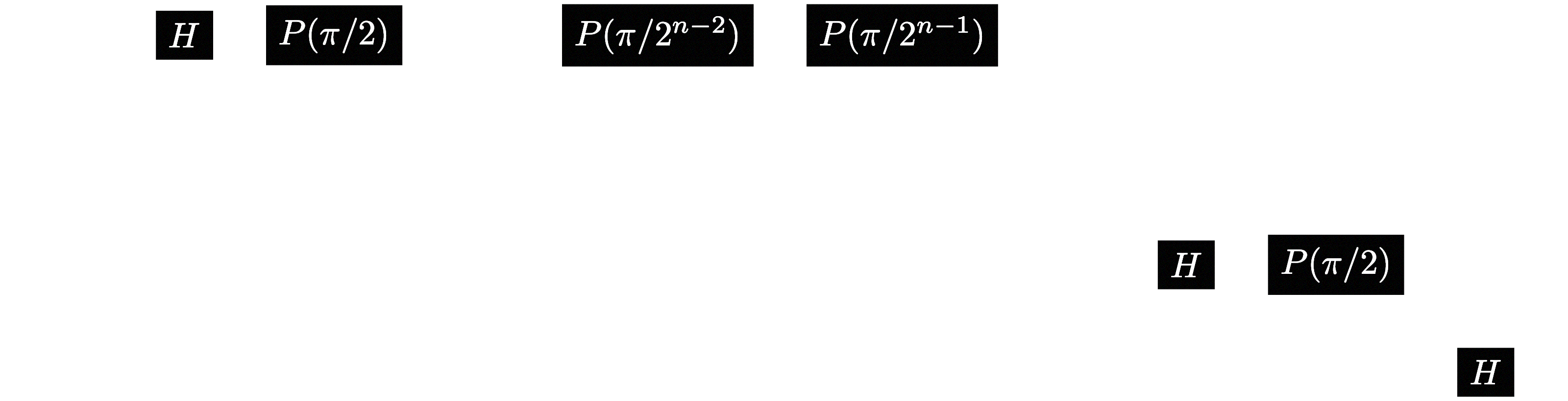
The important thing to remember is that the phase gate parameter always begins at $\pi/2$ and is halved as we go down each qubit.3
While there are built-in QFT functions in most quantum computing software development kits, I think it's important to understand the foundation of how the circuit is constructed.
Of course, the question now is what we can use it for.
Phase Estimation
Suppose we have a unitary operator $U$ and an eigenvector $|v_\phi\rangle$ of this operator. We want to find the eigenvalue associated with this eigenvector. In other words, we want to find the $\phi$ such that
$$ U|v_\phi\rangle = e^{i\phi} |v_\phi\rangle, $$as the eigenvalues of a unitary matrix must have unit norm.
However, we need to be a bit careful, since $\phi$ has period $2\pi$. To get a unique phase, we can define $\phi=2\pi\theta$ where $0 \leq \theta \leq 1$. This will be the unique output we are looking for.
We want to find a circuit that maps
$$ |v_\theta\rangle |0\rangle \to |v_\theta\rangle |\theta\rangle, $$as this allows us to keep the state $|v_\theta\rangle$ throughout the computation of our circuit. The second register, where we store the output, is known as the estimation register.
Now, I have clearly been teeing up the fact that this algorithm will be solved using QFT. We want to construct a circuit such that the number of qubits will dictate the precision of our answer, i.e. we will find that $\theta = j/2^n$ for some output state $|j\rangle$.
To do this, we will apply the QFT in reverse, transforming the state
$$ \frac{1}{2^{n/2}} \sum_{k=0}^{2^n-1} e^{2\pi ijk/2^n}|k\rangle \to |j\rangle. $$Notice that the exponential term is very similar to $e^{i\phi} = e^{2\pi i\theta}$, but with an extra multiple of $k$. We can account for this by applying our unitary $U$ on the eigenvector $k$ times, giving us
$$ U^k |v_\theta\rangle = (e^{i\phi})^k |v_\theta\rangle = e^{2\pi i \theta k}|v_\theta\rangle = e^{2\pi ijk/2^n}|v_\theta\rangle. $$This is exactly what we want! We could just assume that we can construct $U^k$ for $k$ up to $2^n$ and apply each operator onto $|k\rangle$, but it turns out that this isn't a great assumption to make.
It's far more reasonable to assume that we can implement $U^{2^\ell}$ for $\ell$ up to $n$, since squaring a unitary is a far easier operation to implement than applying an arbitrary power.
This is where the logic of the QFT circuit comes in! Let's try to express $\theta$ as a binary decimal, like we did in the QFT circuit. We can do this by setting up a controlled unitary with qubit $s$ as the control and $|v_\theta\rangle$ as the target. The unitary applied will then just be $U^{2^s}$. Therefore, if qubit $s$ is measured as $1$, it will apply the unitary $2^s$ times, leading to its corresponding binary contribution.
We are left with
$$ U^{k_0+2k_1+4k_2+\cdots+2^{n-1}k_{n-1}}|v_\theta\rangle = U^k|v_\theta\rangle, $$which is exactly what we want. Using $U^k$, we can map
$$ \frac{1}{2^{n/2}} \sum_{k=0}^{2^n-1} |k\rangle|v_\theta\rangle \to \frac{1}{2^{n/2}} \sum_{k=0}^{2^n-1} e^{2\pi i\theta k} |k\rangle|v_\theta\rangle, $$and from there apply the inverse QFT to get a final state of $|\theta\rangle$ in the estimation register. To get the initial state, we simply begin with $H^{\otimes n}|0\rangle|v_\theta\rangle$.
As you can guess, if the phase is not exactly a fraction of $2^n$, there will be some error induced in the result. However, it turns out that this error is quite small, and decreases as the number of qubits increase, despite the added cost of applying the unitary operator more.
There are two more points I want to make.
Firstly, I want to note how remarkable it is that this algorithm can find eigenvalues without diagonalizing a matrix. This can allow for much more efficient calculations, especially for large matrices. If you weren't convinced by last week, this is a clear example of the utility of quantum computing. However, quantum hardware isn't quite there yet to compute cases that would be out of reach for classical computers. As time passes and quantum hardware becomes better, though, this will almost certainly change.
Secondly, a limiting factor of this algorithm you may not have thought of is the fact that you need an eigenvector to run the algorithm. It turns out that with a specific setup, you can apply the algorithm even when you don't have a specific eigenvector, using some very clever manipulation and the power of quantum superposition. This is exactly the insight that powers Shor's algorithm—breaking classical encryption as we know it.
1. As we will see, the QFT on one qubit is simply a Hadamard gate.
2. We can perform the QFT for a superposition of terms that isn't a power of 2, but for simplicity, the circuit we will be covering is for $2^n$ terms using $n$ qubits.
3. You may notice that the contributions from qubits farther down the circuit become smaller and smaller. While the circuit requires $O(n^2)$ gates, it can be approximated more efficiently by cutting off the number of phase gates on each qubit at a certain point.